43 pivot table 2 row labels

chandoo.org › wp › quick-tip-rename-headers-in-pivotQuick tip: Rename headers in pivot table so they are presentable Mar 15, 2018 · Pivot tables are fun, easy and super useful. Except, they can be ugly when it comes to presentation. Here is a quick way to make a pivot look more like a report. Just type over the headers / total fields to make them user friendly. See this quick demo to understand what I mean: So simple and effective. towardsdatascience.com › automate-excel-withAutomate Pivot Table with Python (Create, Filter and Extract) May 22, 2021 · After the Pivot Table is created, wb.Save() will save the Excel file. If this line is not included, the Pivot Table created will be lost. If you are running this script to create Pivot Table in the background or on a scheduled job, you may want to close the Excel file and quit the Excel object by wb.Close(True) and excel.Quit() respectively. In ...

Pivot Table adding "2" to value in answer set 1) Right click your pivot table -> Pivot table options -> Data -> Change "Number of items to retain per field" to NONE 2) Wipe all rows in your data source except for the headers 3) Refresh the pivot table 4) Save, and close all instances of Excel 5) Reopen the file, and paste your data 6) Refresh the pivot table

Pivot table 2 row labels

How to repeat row labels for group in pivot table? In Excel, when you create a pivot table, the row labels are displayed as a compact layout, all the headings are listed in one column. Sometimes, you need to convert the compact layout to outline form to make the table more clearly. But in tphe outline layout, the headings will be displayed at the top of the group. Ranking to a Pivot Table with multiple Row Labels I have a pivot table with multiple Row Labels: Team and Player. I created a second Pts column and used 'Show Values As - Rank Largest to Smallest', but it's not working. It's showing up as '1' for all columns, regardless of whether or not I pick 'Team' or 'Player' as the base field. If I remove 'Team' as a Row Label, however, it works perfectly. Combining two+ Columns to form one Row label column in ... Hello, I have multiple sets of data that occur in 2 column increments. The first column is a list of part numbers, the second is their value for that month. I want a pivot table that combines all of the first columns into one master row label of Part numbers and then the values will be listed out in each subsequent column. If a particular month doesn't have a part number in its data, then it ...

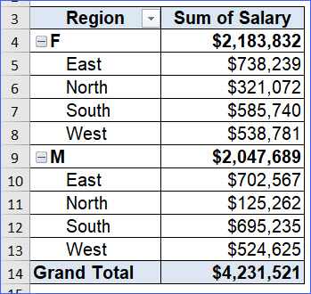
Pivot table 2 row labels. › Add-Rows-to-a-Pivot-TableHow to Add Rows to a Pivot Table: 9 Steps (with Pictures) Feb 15, 2022 · Reorder the field labels in the "Row Labels" section. If you already have a field in the Rows area, adding another row below that will nest the new row within the existing row. [2] X Trustworthy Source Microsoft Support Technical support and product information from Microsoft. excel - Custom row labels in PivotTable - Stack Overflow If you go the pivot table data and right click you can change the value field settings to give a custom name to a row/series but I do not know about individual data points. path: pivot table data => right click => select Field Settings => edit custom name. It does not look like it modifies the raw data (before pivot table). Pivot Table Sort by second row label - Microsoft Community Replied on May 17, 2014 Here is how you can get the results: Place your cursor on Col. B data wherever Names are. Goto Home ribbon>Editing>Sort it in either way. Alternatively, you can Sort from Pivots settings. Ramz Aftab [ MOS 77-888/82 Excel Expert ] ramzaftab [at]gmail [.]com Report abuse Was this reply helpful? Pivot table row labels in separate columns • AuditExcel.co.za So when you click in the Pivot Table and click on the DESIGN tab one of the options is the Report Layout. Click on this and change it to Tabular form. Your pivot table report will now look like the bottom picture and will be easier to use in other areas of the spreadsheet and in our opinion is also easier to read.

How to Use Excel Pivot Table Label Filters To change the Pivot Table option to allow multiple filters: Right-click a cell in the pivot table, and click PivotTable Options. Click the Totals & Filters tab Under Filters, add a check mark to 'Allow multiple filters per field.' Click OK Quick Way to Hide or Show Pivot Items Easily hide or show pivot table items, with the quick tip in this video. How to Add Two-Tier Row Labels to the Pivot Table in ... Step 2: Click Add button on the Rows header in the Pivot table editor sidebar. Pivot table editor sidebar, Add button besides Row label encircled. ‍ A drop-down box of the list of columns will appear. Select the column you want to use. For our case, we want to select the date column. How to make row labels on same line in pivot table? Make row labels on same line with setting the layout form in pivot table As we all know, the pivot table has several layout form, the tabular form may help us to put the row labels next to each other. Please do as follows: 1. Click any cell in your pivot table, and the PivotTable Tools tab will be displayed. 2. Gallery of 33 pivot table blank row label labels database ... 33 Pivot Table Blank Row Label Labels Database 2020 images that posted in this website was uploaded by Film.norden.org. 33 Pivot Table Blank Row Label Labels Database 2020 equipped with a HD resolution 687 x 377.You can save 33 Pivot Table Blank Row Label Labels Database 2020 for free to your devices.. If you want to Save 33 Pivot Table Blank Row Label Labels Database 2020 with original size ...

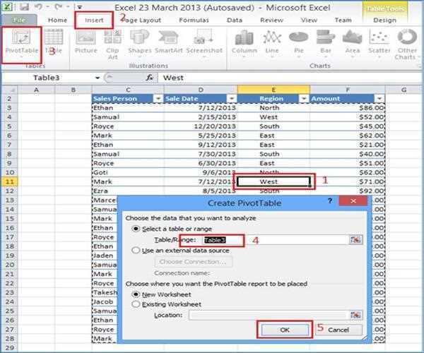
› excel-pivot-taHow to Create Excel Pivot Table [Includes practice file] Jan 15, 2022 · The area to the left results from your selections from [1] and [2]. You’ll see that the only difference I made in the last pivot table was to drag the AGE GROUP field underneath the PRECINCT field in the Row Labels quadrant. How to Create Excel Pivot Table. There are several ways to build a pivot table. Pivot Table "Row Labels" Header Frustration - Microsoft ... Hi Everyone please help I can't change my headers from Row Labels in a Pivot Table. Using Excel 365 Pivot Table Row Labels | MrExcel Message Board I am trying to get a pivot table to show the row labels on each row, not just the top row as they usually do. I have 2 separate companies and it shows the company numbers, 12 and 88 once, where each company starts. I need it to show the 12 on each row that is applicable to that company... How to rename group or row labels in Excel PivotTable? 1. Click at the PivotTable, then click Analyze tab and go to the Active Field textbox. 2. Now in the Active Field textbox, the active field name is displayed, you can change it in the textbox. You can change other Row Labels name by clicking the relative fields in the PivotTable, then rename it in the Active Field textbox.

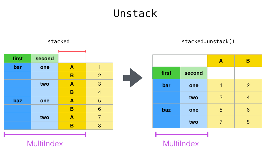
Reshaping and pivot tables — pandas 1.0.3 documentation

Pivot table row labels side by side - Excel Tutorials You can copy the following table and paste it into your worksheet as Match Destination Formatting. Now, let's create a pivot table ( Insert >> Tables >> Pivot Table) and check all the values in Pivot Table Fields. Fields should look like this. Right-click inside a pivot table and choose PivotTable Options…. Check data as shown on the image below.

Pivot Table in Excel

Multi-level Pivot Table in Excel (In Easy Steps) First, insert a pivot table. Next, drag the following fields to the different areas. 1. Order ID to the Rows area. 2. Amount field to the Values area. 3. Country field and Product field to the Filters area. 4. Next, select United Kingdom from the first filter drop-down and Broccoli from the second filter drop-down.

How to Increase Indent Row Labels in Pivot Table Compact Form - ExcelNotes

blog.hubspot.com › marketing › how-to-create-pivotHow to Create a Pivot Table in Excel: A Step-by-Step Tutorial Dec 31, 2021 · Step 4. Drag and drop a field into the "Row Labels" area. After you've completed Step 3, Excel will create a blank pivot table for you. Your next step is to drag and drop a field — labeled according to the names of the columns in your spreadsheet — into the Row Labels area. This will determine what unique identifier — blog post title ...

Show Text in a Pivot Table Values Area - Excel Pivot TablesExcel Pivot Tables

How to Customize Your Excel Pivot Chart Data Labels - dummies To add data labels, just select the command that corresponds to the location you want. To remove the labels, select the None command. If you want to specify what Excel should use for the data label, choose the More Data Labels Options command from the Data Labels menu. Excel displays the Format Data Labels pane.

pivot table - Excel PivotTable Remove Column Labels - Super User

pivot table how to combine 2 row labels | MrExcel Message ... Nov 6, 2013 #1 Hi, i am having the pivot table in the below format. my concern is how i can combine both A & AA together the source is from data connection and not from the excel. This is pivot table output, my request is it possible to combine A & AA together in existing pivot table Look Like this:

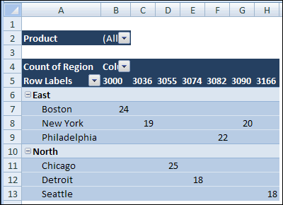
excel pivot table - multiple columns - Stack Overflow

get a row label from pivot table - Microsoft Tech Community I am not a great Pivot Table user so I tend to duck out of the PT environment and resort to dynamic arrays. = UNIQUE(Table1[Medewerker]) If you also wish to filter the headings to omit the rows without content the formula starts to get somewhat overcomplicated.

vba - Extracting "hidden" data from expanding/collapsing pivot table - Excel - Stack Overflow

How to add side by side rows in excel pivot table ... First, you have to create a pivot table by choosing the rows, columns and values: Created pivot table should look like this: You have to right-click on pivot table and choose the PivotTable options. Then swich to Display tab and turn on Classic PivotTable layout: Now the pivot table should look like this: As a next step, you have to modify the ...

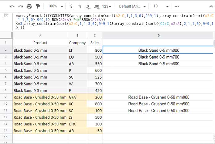
Filter Top 3 Values in Each Group in Pivot Table - Google Sheets

Pivot Table Row Labels In the Same Line - Beat Excel! Now click on "Error Code" and access field settings. First check "None" option in "Subtotals & Filters" tab to disable totals after every row. Then navigate to "Layout & Print" tab and click on "Show item in tabular form" option. Do this procedure also for "Dealer" field and your table will look like this:

Share :